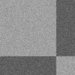
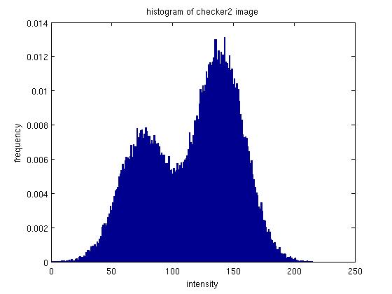
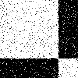
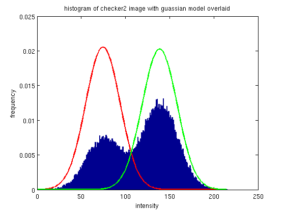
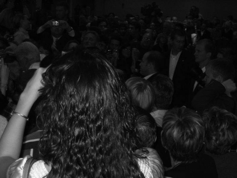
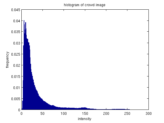
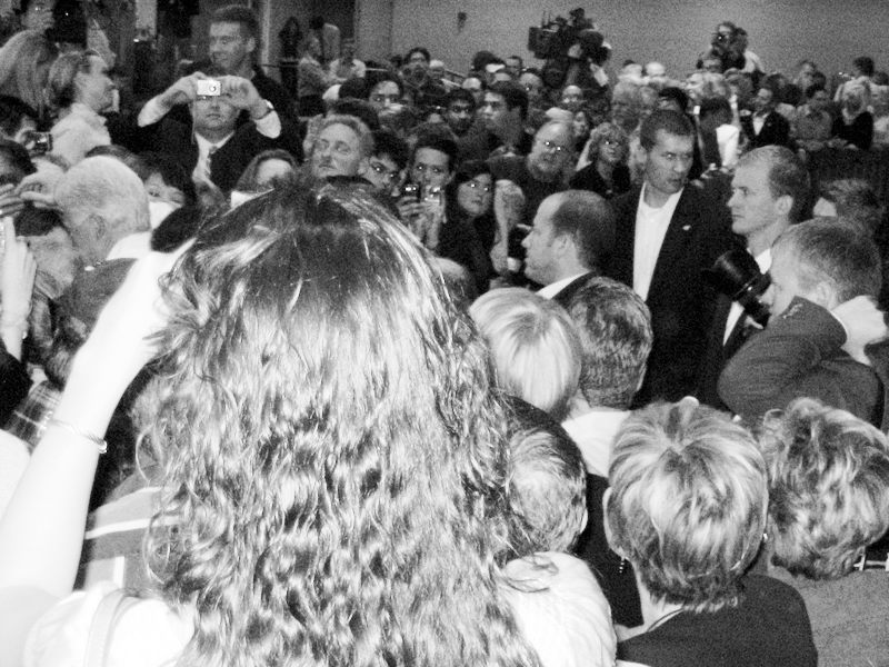
Histograms

Histograms

code:

examples:

This example shows histogram is take from the "crowd.tif" image included in the assignment. The histogram shows a high concentration of lower-intensity pixels. This makes sense when you look at the image, as it is a very dark image, with a lot of low-intensity pixels.
This example shows histogram is take from the "checker1.gif" image included in the assignment. The histogram shows two large concentrations of pixel intensitys, each with a guassian-like distribution. Again, this makes sense looking at the picture, as the image appears to contain two main intensity values, with each intermixed with some type of noise.
This example is my own photograph. The histogram shows a pretty large range of intensity distributions, with two dominating peaks - one at the highest intensity, around 250, and the other at around 50 - a darker grey. These make a lot of sense looking at the photograph, as there is a large collection of white clouds in the sky - contributing to the large number of intensities around 250. The other peak around 50 is probabyl due to the grey intensities of the mountains, which make up a large part of the photograph.
This example is also one of my own photographs. This histogram also shows a wide distribution of values. It's a little more difficult to draw exact relationships between picture elements and peaks in the histogram, but it is easy to see that the majority of the intensities exist in the mid-range of intensity values - and correspondingly most of the image is in the mid-range of intensities - ie there aren't many very white or very black areas. Overall the histogram does make sense.

Histogram Equalization

code:

examples:


"crowd"

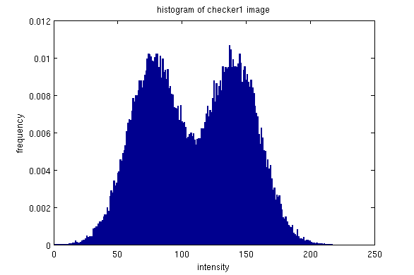
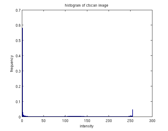
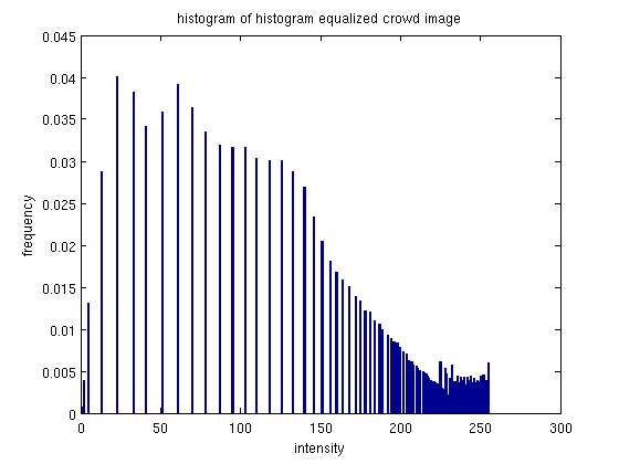
In this image, the histogram of the original image shows a larg clustering of images on the far left - which corresponds to the overall low intensity of the image. After histogram equalization, the histogram density appears to have spread out over the intensity spectrum. It also seems to have space out the different intensity values represented: in the original histogram the bars are close enough to appear contiguous, while in the equalized histogram, the bars are not only more evenly distributed, but also more spaced.

The effect on the image is very obvious - with a more diversified spread of intensities, the image appears much more bright as compared to the original. The equalizatino hasn't just brightened pixels, it has give a more even spread of intensities, so that the image has more brightness and contrast.


"university"

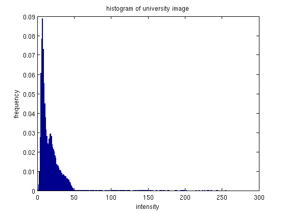
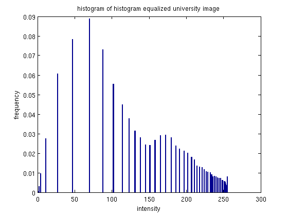
This image is similar to the first, in that the original histogram has a dense clustering of intensities on the low intensity end. Again after equalization these intensities spread out. It's also interesting to note that there is actually a more dense clustering of pixels on the opposite (high intensity) end of the intensity spectrum than, and a much sparser clustering of intensity on low intensity end.

The image after equalization again looks brighter as compared with the original. With the better spread of intensity values, one can see more details that were previously blended in the low intensity lump. One detail that is hard to see without zooming in on the images, is that while teh equalized image looks good overall, the image appears more grainy. However this detail could probably be taken care of with some amount of gaussian smoothing - as evidenced by it not being noticeable except when zoomed in.
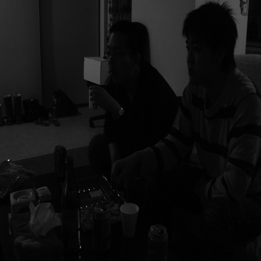
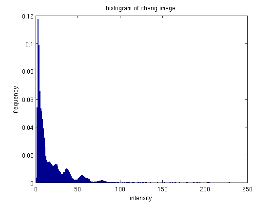
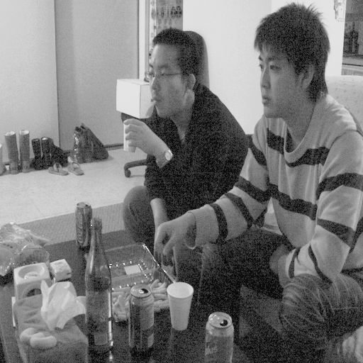

"chang"

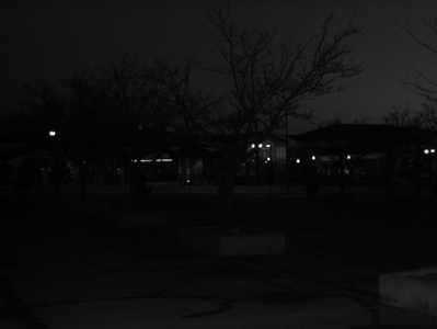
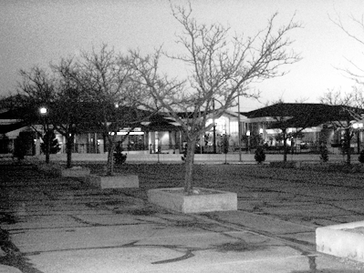
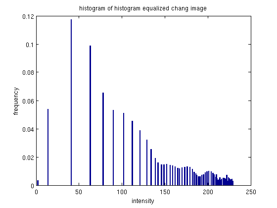
This image was also original quite dark, and consequently the original histogram is very clumped at the low-intensity end. After equalization the histogram mass has been spread out across the intensity spectrum. Again, there appears to be some clumping of the intensities on the high intensity end.

The equalized image has the expected result, it appears more clear and details are more discernible than the original. The better spread of intensities allows for more contrast and brightness variety than in the original image.


"portal"

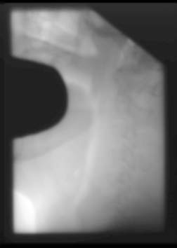
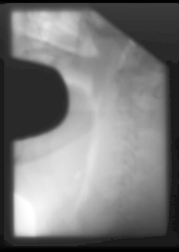
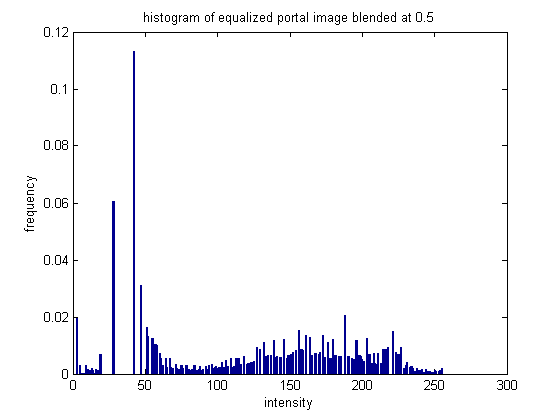
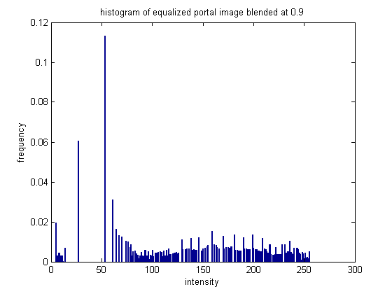
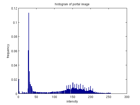
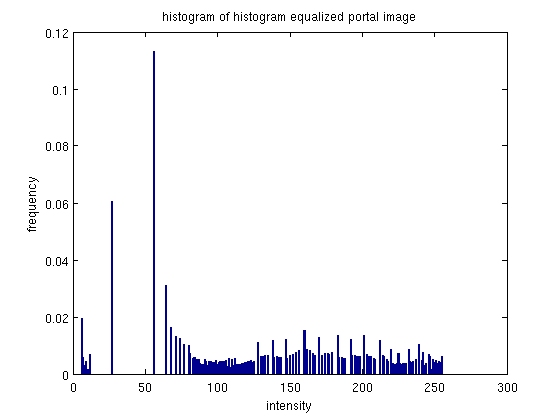
This image didn't have a huge change in the histogram. The original histogram was already fairly spread out, the equalized histogram has a little more distance between some of the bins.

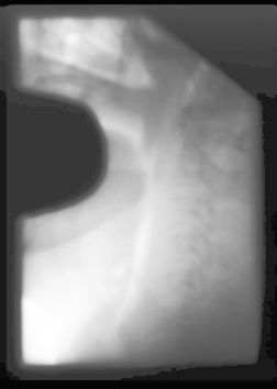
The image also did not change a lot, but did change some. Specifically, some of the detail in the middle of the lighter area is now visible, and you can almost make out some sor tof bone structure. The equalization was not quite as effective for this image, because the histgoram was already fairly well distributed.
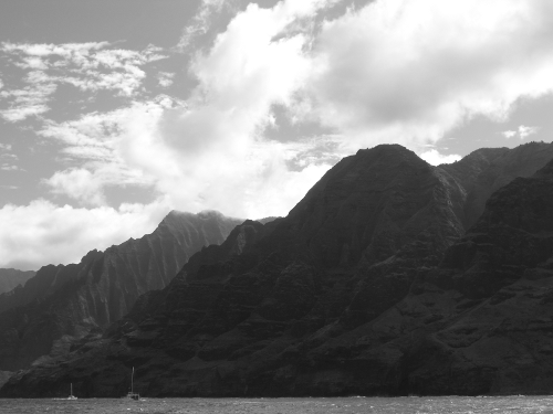

"napali"

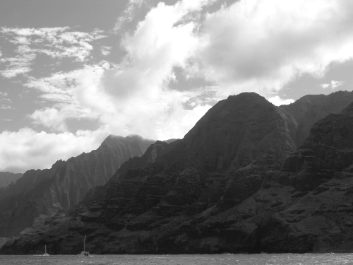
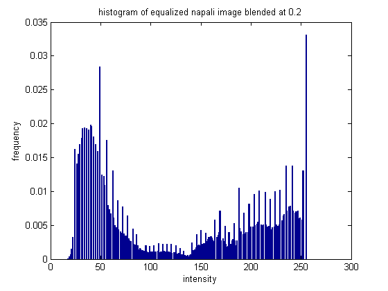
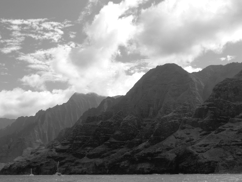
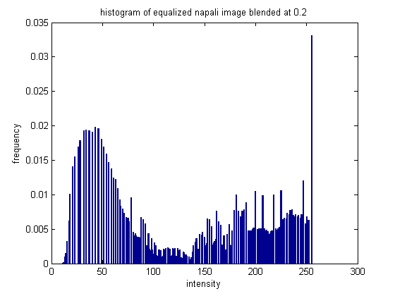
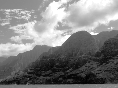
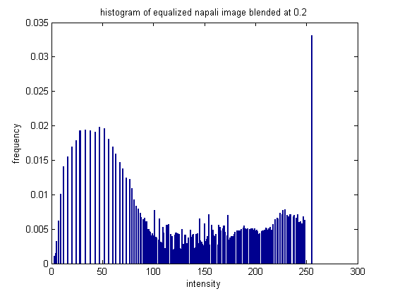
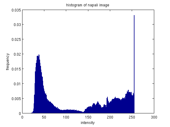
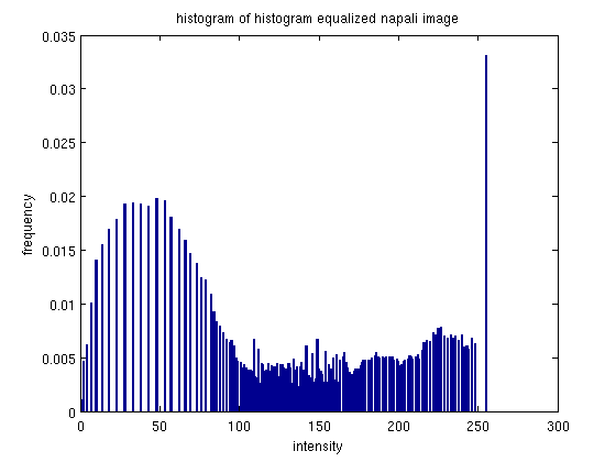
This is an interesting picture to see how histogram equalization works, because the image includes a large group of really bright pixels (clouds), and a large group of lower/mid-intensity pixels (mountains). The equalization is able to break up and spread out the intensities a little more.

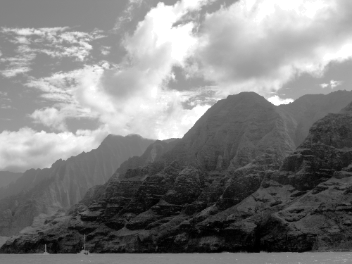
The image has noticeable changes - the darkened moutains appear to have a more lustery surface, although the effect almost looks like snow. While the equalization had some effect, it appears that because of this specific scene the effects are not preferable.. the original image is probably better. Thist is one of the pictures we will be using the blending histogram equalization approach on below.
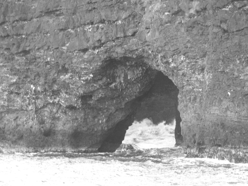
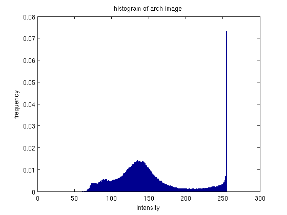
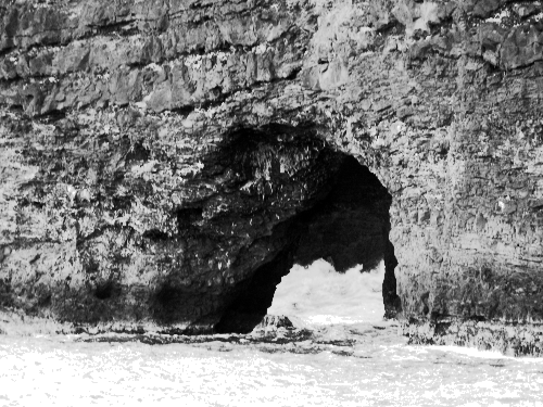
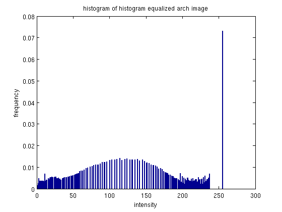

"arch"

Again, this image contains a large group high-intensity pixels (wave crests, and reflection off the water) and a large group of mid to low-intensity pixels (rock making up the arch). The histogram again spreads out the histogram by incorporating more dark intensity pixels It also seems to have groups and spaced the pixels - resulting in a sort of smoothing over of a small bulge in the middle of the histogram.

The effect of the equalization on the image is not very desirable. While the details in the rock crackers are more observable, this isn't very good in a visual sense. The waves appear more washed out as well. The equalization didn't have a very good effect because the pixels were already pretty well spaced, and probably also due to the pixels having two large groups - bright and mid-range... making it difficult to evenly spread them.
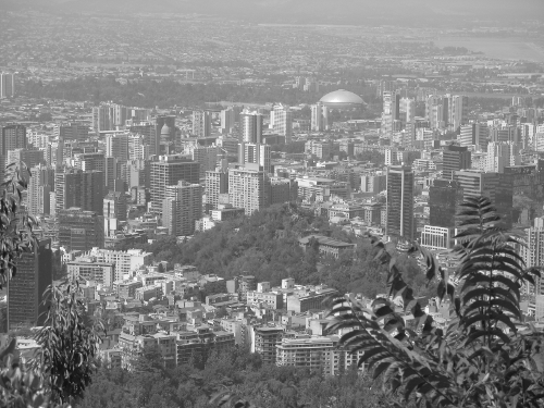
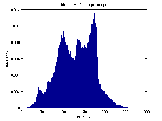
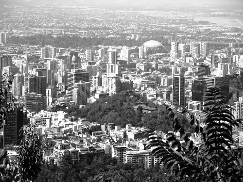
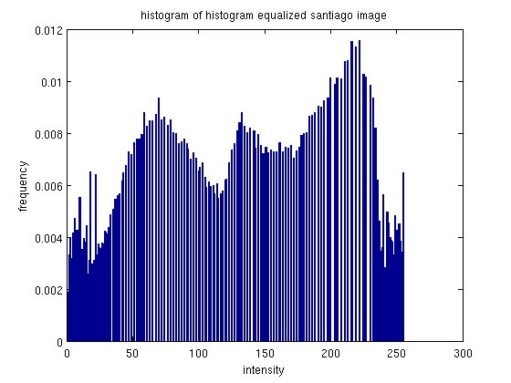

"santiago"

While this histogram has a good range of values, there is also some clumping to the center of the histogram. The majority of the mass of the histogram is in the center. Equalization spreads that mass out more evenly across the intensity spectrum, giving a more balanced look to the histogram.

The effect of this on the image actually very good. While the original seems a little over-exposed, giving an almost hazy feel to the city-scape, the equalized image looks more sharp and crisp. The buildings in the image also appear more bright, and the vegetation up close looks more dark. In the original both were a little more mid-intensity which made the image dull.

Blended histogram equalization

code:

examples:

I decided to use two images in this example that were difficult to look good equalized, in hopes that with some blending the result coudl be improved. The "portal" and "napali" images from above are show below with differing blends of histogram equalization.

"portal"

The above images show (from top) the original portal image, followed by a histogram equalization blended with alpha = 0.2, 0.5, 0.9, and the fully equalized image (alpha = 1.0). As the images increase alpha from 0.0 to 1.0, the histogram slowly changes from a more compact histgogram to a slightly more spread out histogram.

The images also show a noticeable transition from the original to a fully equalized image. In the original it is difficult to see any details, while in the fully equalized image, one can make out some forms of a skeleton. By blending with the original we recapture some of the original pixel distrubtion, which softens slightly some of the effects of this image. In this situation the softening effect probably isnt' desirable, as the goals is to make out the details of the scan. However the next example does show desirable benefit from this technique.


"napali"

The ordering of the histograms above provides for a view into the transition of the histogram from the original to a more dispersed, equalized histogram. By slowly moving the eye from one to the other you can almost see the sharp peak on the left melt into the rounded hill in the equalized image.

The images also display a transition from original to equalized. As noted in the equalizaiton discussion above, the equalized version of this image isn't very visually appealing, as the equalization gives the mountains a glazed effect, making it almost look like snowy peaks. By blending the equalized histogram with the original, this effect can be softened. For example the image associated with alpha = 0.2 appears to have a more contrast in the details of the mountain (more than the original), but doesn't go overboard in highlighting the moutain surfaces - it appears to be a good balance of enhancement and original image.


code:

examples:

"checker1"
Selecting threshold visually:

The histogram of the "checker1" image is shown above. Visually inspecting the histogram in matlab (using the data picking tool), I found the intensity of 110 to be a good separator of the two distributions. The results of using that value to threshold the original image is show above. As can be seen the threshold seems to have worked pretty well.

Selecting threshold with a simple model:

By modeling the distribution of pixels in both the light (mean=140.50, stdev=20.00) and dark (mean=76.33, stdev=20.15) regions we are able to estimate the intersection of the two models: 108.42. These distributions have been plotted on top of the histogram of the images above right, to give you an idea of how well they match. That threshold was then used to segment the image, which is show above left. The threshold estimate was made by averaging the means of the two distributions - which works in this case becase the standard deviations are so similar.


"checker2"
Selecting threshold visually:

The histogram of the "checker2" image is shown above. Visually inspecting the histogram in matlab (using the data picking tool), I found the intensity of 103 to be a good separator of the two distributions. The results of using that value to threshold the original image is show above. As can be seen the threshold seems to have worked pretty well.

Selecting threshold with a simple model:

By modeling the distribution of pixels in both the light (mean=138.66, stdev=19.69) and dark (mean=74.48, stdev=19.42) regions we are able to estimate the intersection of the two models: 106.57. These distributions have been plotted on top of the histogram of the images above right, to give you an idea of how well they match. That threshold was then used to segment the image, which is show above left. The threshold estimate was made by averaging the means of the two distributions - which works in this case becase the standard deviations are so similar.


"ctscan"

Selecting threshold visually:

The histogram of the "ctscan" image is shown above. Visually inspecting the histogram in matlab (using the data picking tool), I found the intensity of 103 to be a good separator of the two distributions. The results of using that value to threshold the original image is show above. As can be seen the threshold seems to have worked pretty well.


Selecting threshold with a simple model:

By modeling the distribution of pixels in the bone (mean=253.71, stdev=2.15) and tissue (mean=118.15, stdev=12.37) regions we are able to estimate some meaningful separation of the two models: 185.93, and of the tissue model with everything else: 59.07. These distributions have been plotted on top of the histogram of the images above right, to give you an idea of how well they match. Those thresholds were then used to segment the image, which is show above left. We didn't explicitly model the non-tissue,non-bone pixels, except to say that they were close to 0, which we used when computing the separating threshold betwen the tissue mean and the other pixels. The separation between the bone mean and tissue mean was computed using the mean of those values. While the distrubtions didn't have similar standard deviations, a mean seemed a decent way of calculating a fair division between the two.


(code can be found here.)